Hi, nerds !

Let’s say that you (like me) have just learned basics of probabilistic programming – you have some ideas why it’s usefull and you tried some things using existing libraries.

Now you wonder – how the hell does it actually work ? Let’s go deeper !

I am writing this primarily to myself to structure my knowledge. Goal is to test it on an example and also kill several buzzwords and replace them with intuition your grandma could understand

Monte Carlo
Markov Chain
Monte Carlo Markov Chain (MCMC)
Metropolis-Hastings

The problem

Let’s say you have described phenomenon with fancy model using probability distributions. It might be movement of stock, result of portofolio after some time, weather or something else.

We will start with something very simple – one Gaussian

$$X \sim \mathcal{N}(\mu,\sigma^2)$$

This might represent something natural – something where extremes are less and less likely – height or weight or person etc

You might have some examples of data and you will not know what is the “generator” distribution as it will be nature, god or crazy people on stock market. At this point (depending on what’s your goal) you might want to know values of variables/hyperparameters of your model, which best describes the data you have.

Let’s generate some data – mean is 5 and variance is 1

1 2	`data = np.random.normal(5, 1, 500) plt.hist(data)`

Generated data

Now, we want to find values of $\mu$ and $\sigma^2$

Of course we could simply compute mean and standard deviation from the data we have, but in reality, the model will be much more complex than one normal distribution

To make it even more simple, let’s forget about $\sigma^2$ and say that we know it (it’s 1)

Probabilistic programming is using bayes theorem to find most probable value of our hyperparameters ($\theta$) with

Some example data we are trying to describe by model – $X$
Some prior belief what those hyperparameters might be $P(\theta)$

$$P(\theta∣X)= \frac{P(X)P(X∣\theta)}{P(\theta)}$$

This equation will not give us single value of $\mu$, but probability distribution – values of $\mu$ which when used as mean of gaussian better describe data we have and at the same time are more likely given our prior belief what those values should be, will be more likely

So once again – our goal is not to approximate distribution of $X$ but rather approximate posterior distribution of $\theta$(from which we care only about $\mu$ for simplicity)

So let’s try to compute it

likelyhood – $P(X|\theta)$ – if the parameter would be like that, how does it explain the data we have.

1	`scipy.stats.norm(mu, 1).pdf(data).prod()`

prior – $P(\theta)$ – is such parameter likely given our prior belief about what our variable might be. Easy to compute

1	`scipy.stats.norm(prior_mu, std).pdf(mu)`

evidence or normalization factor – $P(X)$ – is probability, that data we have was generated by the model (all possible parameters $\theta$). This one is tricky as we would need to evaluate all possible distributions (of same class). This is equivalent to computing integral $\int {P(x,\theta)\delta\theta}$ This is possible for simple distributions, but with more complex with more variables it would be extremely hard – we need a trick around that

One does not simply sample everyting

Metropolis Hastings

Metropolis-Hastings is algorithm able to indirectly sample from posterior distribution. It works by creating “shadow” distribution which is proportional to distribution we want to sample from. This “shadow” distribution becomes more and more like the target distribution as we sample from it.

The algorithm is as follows:

make initial guess about shadow distribution
take first value from shadow distribution
for a loong time:
  randomly propose value of param from shadow distribution
  compute how 
     - new value fits to prior belief about it
     - old value fits to prior belief about it
     - data fits to distribution described by new value
     - data fits to distribution described by old value
  if new value "better fits" then old value
    shift shadow distribution towards new value
  else
    shift shadow distribution towards old value

The condition is not that strict, new value will be used in proportion to new_fit/old_fit – even if new value is worse than old, it will be used some of the time – this ensures it will not stuck in local maximum

We choose “better fitting” value relatively more often than the “worse fitting” value

$$ \frac{\frac{P(x|\mu_t)P(\mu_t)}{P(x)}}{\frac{P(x|\mu_0)P(\mu_0)}{P(x)}} = \frac{P(x|\mu_t)P(\mu_t)}{P(x|\mu_0)P(\mu_0)} $$

If we put posteriors of both “good and bad” suggestions to proportion, we can see, that it’s the same whether we use posterios (normalized by P(x)P(x)) or not. This means that that the “shadow” distribution is proportional to posterior distribution we are looking for. Why ? Because good vs bad values in shadow distribution are as likely as good vs bad values in posterior distribution (see the equation) and we made sure, that good fits are more likely than bad fits

Let’s build it 🙂

We are going to sample from shadow distribution and remember each value so we can later visualize it.

iterations = 200
prior_mu = 1 # Let's purposely choose bad value (it should be 5)

dtype = [
    ("posterior", np.float64), # Chosen value of mu variable
    ("current", np.float64), # Previous value of mu variable
    ("proposed", np.float64), # Proposed value of mu variable
]
trace = np.full(iterations, 0, dtype=np.dtype(dtype))

current_mean = prior_mu
std = 2

for i in range(iterations):
    # Propose new mean of "shadow" distribution by sampling from current "shadow" distribution
    proposed_mean = np.random.normal(current_mean, std)

    # How much is current/proposed mean probable given prior
    # Remember that prior is our belief about hyperparameter, not data
    # The fact that prior is gaussian is just coincidence
    prior_current = scipy.stats.norm(prior_mu, std).pdf(current_mean)
    prior_proposal = scipy.stats.norm(prior_mu, std).pdf(proposed_mean)

    # How well are data described by current distribution
    likelyhood_current = scipy.stats.norm(current_mean, 1).pdf(data).prod()
    likelyhood_proposal = scipy.stats.norm(proposed_mean, 1).pdf(data).prod()

    # Suggested distribution both describes data and prior could describe the chosen hyperparameter
    fit_current = prior_current * likelyhood_current
    fit_proposal = prior_proposal * likelyhood_proposal

    # Compute ratio - "how much is new setting better"
    ratio = fit_proposal / fit_current

    trace["current"][i] = current_mean
    trace["proposed"][i] = proposed_mean

    # Probability of accepting new parameter is proportional to "how better it is"
    # Even if it completely sucks it will be used time to time
    # This will ensure, that we will not stuck in local minimum
    if ratio > np.random.rand():
        current_mean = proposed_mean
        trace["posterior"][i] = proposed_mean
    else:
        trace["posterior"][i] = current_mean

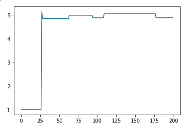
If we plot the trace, we will see that it converges to 5. The steps until it happens is called burn-in period

1	`plt.plot(np.arange(trace["current"].size), trace["current"])`

$Evolution of \mu value$

It would be even more clear if we animate it

fig, ax = plt.subplots(1, 3, figsize=(20, 10))
fig.set_tight_layout(True)

ax1_twin = ax[1].twinx()

def update(i):
    if i > 0:
        ax[0].clear()
        ax[1].clear()
        ax1_twin.clear()
        ax[2].clear()

    # Draw prior
    # Prior does not change, only the mean we choose
    ax[0].set_title("Prior (match on what we thought)")
    mu = 1
    variance = 20
    sigma = math.sqrt(variance)
    x = np.linspace(mu - 3*sigma, mu + 3*sigma, 100)
    ax[0].plot(x, scipy.stats.norm.pdf(x, mu, sigma), color="blue")

    ax[0].axvline(trace["current"][i], color='b', label="Current")
    ax[0].axvline(trace["proposed"][i], color='r', linestyle='--', label="Proposed")
    ax[0].set_ylabel("Probability density")
    ax[0].set_xlim(mu - 3*sigma, mu + 3*sigma)
    ax[0].legend()

    ax[1].hist(data, alpha=0.5, color="b")
    mu = trace["proposed"][i]
    variance = 1
    sigma = math.sqrt(variance)
    x = np.linspace(mu - 3*sigma, mu + 3*sigma, 100)

    ax1_twin.plot(x, scipy.stats.norm.pdf(x, mu, sigma), color="red", label="Proposal")
    ax1_twin.legend()
    ax[1].set_xlim(0, 10)
    ax[1].set_title("Likelyhood (match on data)")

    ax[2].set_title("Posterior (of variable mu)")
    ax[2].plot(np.arange(i), trace["posterior"][:i], label="Development of variable")
    ax[2].axhline(np.mean(trace["posterior"][:i]), color='r', linestyle='--', label="Mean of iterations")
    ax[2].legend()
    ax[2].set_xlabel("Iterations")
    ax[2].set_ylim(0, 10)

anim = FuncAnimation(fig, update, frames=np.arange(0, 120), interval=500)

Left-most column shows prior (it’s static) and current (best) and proposed value (proposed mean of distribution of $\mu$)
Middle column shows data we have (blue) and proposed gaussian describing that
Right column visualizes the trace and displays mean – the mean converges to real value of $\mu$ (5)

Now let’s just save it as .gif file, wait one lifetime until it happens and see

1	`anim.save('metropolis.gif', writer='imagemagick', fps=5)`

$Metropolis-Hasting convergence of \mu vale$

You can see, that we are struggling for some time (burn-in period) before converging. It’s because we have chosen bad value of our prior – we have chosen 1 and by that making the truth value 5 an unlikely sample. So choice of prior might speedup/slowdown the convergence (unless the right values has probability of 0)

Let’s kill the buzzwords:

Monte Carlo – more or less stupid brute force over some sample space to find what we are looking for
Markov Chain – random walk – step $t_n$ depends only on $t_{n-1}$ fancy people call this "markov blanket" Where is markov chain hidden in Metropolis-Hastings ? In shadow distribution ! Based on current value, we will draw new one, which will either be next value or not
Monte Carlo Markov Chain – combination of the two above for example using Metropolis-Hastings
Metropolis Hastings – specific implementation of MCMC (not the smartest)

If you managed to read so far, I would like to congratulate – you can now explain MCMC to your grandma.

If you found any mistakes or have any suggestions about the article, please let me know in comments